
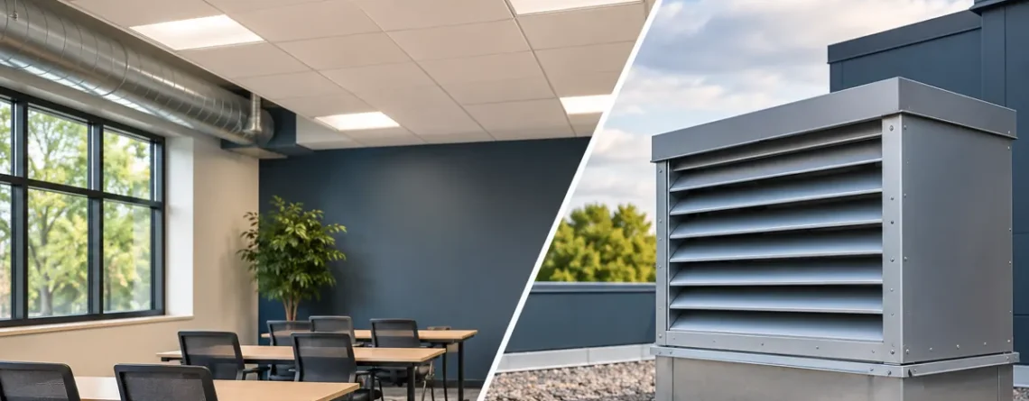
The indoor–outdoor CO₂ difference is the indoor reading minus the concentration of the outdoor air entering the space, expressed in ppm. A room at 1,050 ppm with an intake at 450 ppm has an excess of 600 ppm for that paired observation. The difference describes the accumulation above incoming background. To use it to estimate outdoor airflow, the room, source and ventilation must also satisfy the assumptions of the calculation.
The same indoor reading can have different meanings with different outdoor backgrounds. The same indoor–outdoor difference can also occur in two rooms with different occupant activity and airflow. Use the difference first as a paired observation. Advance to an airflow estimate only when the air paths, time history and source assumptions support one.
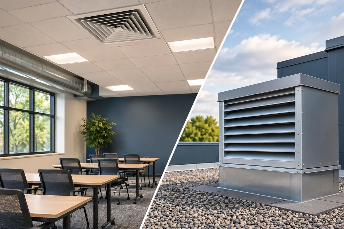
The indoor sample and the outdoor reference describe two different air masses. Take both readings for the same operating interval.
Pair the indoor reading with the air that actually enters
Choose a representative indoor location for the zone being assessed. A room monitor exposed to a jet, an opening or a nearby person's breath can produce a reading that is accurate for its inlet and unsuitable for describing the room. In a large or stratified room, compare multiple occupied locations before choosing a representative value. Identify whether the task is to describe conditions where people sit, characterize a return stream or evaluate a specific mechanical ventilation system.
For a mechanically ventilated room, an outdoor reference should correspond to the intake serving the room. An air quality station across town may describe regional conditions while missing a local plume near that intake. A street-level reading may be unrepresentative of a roof intake. Conversely, a monitor at roof height can miss air entering through a ground-floor entrance. Document where the incoming air originates and whether different paths are active during the observation.
Avoid mistaking exhaust contamination for the ordinary background. If exhaust re-enters an intake, a sample at the intake may accurately capture the air being drawn in while revealing a separate ventilation defect. A comparison between a sheltered upwind location and the intake can help identify the source of a local rise. For the immediate mass balance, use the concentration of the incoming stream if it can be sampled reliably. For diagnosis, retain the second outdoor observation as a separate point.
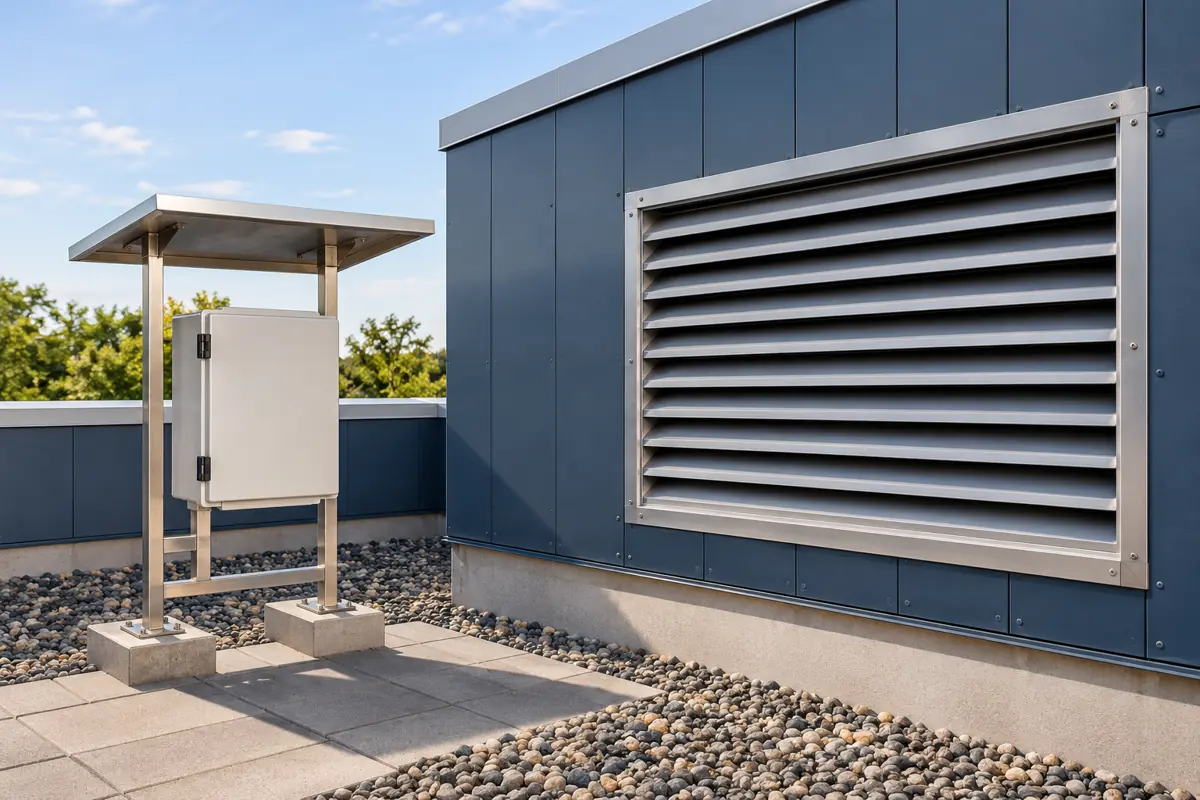
Identify which intake serves the room and note nearby exhausts or combustion sources before choosing the reference.
A fixed background can be appropriate in a specifically approved control or modeling procedure. For an investigative field comparison, a concurrent measurement avoids assuming that background stayed constant between visits. If only a fixed background is available, identify it as assumed and calculate the effect of a plausible change. Suppose the indoor value is 1,050 ppm. At assumed outdoor values of 420 and 550 ppm, the excess is 630 and 500 ppm, respectively. If all else were equal in a steady-state calculation, the estimates based on those differences would differ by a factor of 630/500, or 1.26.
Align the sampling and measurement systems
Set the same clock for both instruments and preserve their native timestamps. Document whether the logging software stores the start, midpoint or end of an averaging interval. A one-minute value labeled with the beginning of its interval will pair differently with a five-minute value labeled with the end. If a building system stores values only on change, determine whether a long flat trace represents a steady signal or merely sparse updates.
Use sufficiently matched response times for the events being analyzed. Outdoor concentrations near a loading area may vary faster than an indoor wall sensor reports. A comparison based on matched averaging windows may be more meaningful than subtracting nominally simultaneous display numbers. Keep the original traces available so a brief local event remains visible. If a common instrument samples both streams through valves or tubing, record each sample's actual time and allow each path to stabilize after a switch.
A pretest collocation can reveal relative offset. Place the indoor and outdoor instruments together in stable air under suitable conditions, wait for them to settle, and compare multiple intervals. Repeat after the test when feasible. A field collocation can show relative agreement at that concentration and under those conditions. Checking agreement at a second relevant concentration or against an appropriate reference answers a broader question about span and absolute performance.
Understand the one-zone mass balance before inverting it
For a well-mixed zone, let V be room volume, Q the outdoor exchange flow, G the total indoor CO₂ generation rate, C the indoor volume fraction and Co the entering outdoor fraction. Under the simplified assumptions of constant volume, balanced air exchange, no other air streams and no significant sinks, the relationship is V × dC/dt = G + Q × (Co − C). Use compatible units for volume and time. To use concentration values in ppm with the equation, convert them to fractions, or include the factor of one million explicitly.
At steady state, the accumulation term V × dC/dt is zero. Rearranging gives C − Co = G/Q as a volume fraction. If ΔC is entered as a number in ppm, the corresponding estimate is Q = 1,000,000 × G / ΔC. When all occupants can reasonably be assigned the same mean generation g and all relevant generation is from occupants, Q per person is 1,000,000 × g / ΔC. The NIST Technical Note on its indoor CO₂ metric tool gives the dynamic equation and explains the influence of occupant characteristics on generation.
The well-mixed assumption concerns both the sample and the concentration of the air leaving the control volume. With several incoming streams at different concentrations, their individual flow and concentration contributions belong in the balance. Transfer air from a corridor can carry CO₂ from elsewhere. Mechanical outdoor air and infiltration at the same concentration may behave as one effective outdoor exchange term in the simplified calculation, but the result cannot say how much came through the mechanical intake.
Recirculation within a well-mixed zone and unchanged CO₂ on its return can cancel out of the zone balance. Air transferred through another occupied zone brings a different composition. A mixed supply duct concentration is likewise distinct from the outdoor reference. Do not substitute supply CO₂ for outdoor CO₂ in a formula whose unknown is outdoor air exchange. A balance using a measured supply concentration and a suitable return concentration can answer a different question under its own assumptions.

Occupant number and activity determine the assumed source term. A headcount alone does not describe generation.
Worked example with stated assumptions
Take a hypothetical room with six occupants, each assigned 0.0045 L/s CO₂ generation for this calculation, and a concurrent excess of 600 ppm. Assume constant occupancy and activity, a stable incoming outdoor concentration, a representative well-mixed volume, no other sources or sinks, no transfer-air contribution and near-steady conditions. The total generation is 6 × 0.0045 = 0.027 L/s CO₂. Divide by 600 × 10⁻⁶ to obtain 45 L/s outdoor exchange, or 7.5 L/s per person. The generation rate is a selected example input. Actual activity, age, body size and related assumptions affect the calculation.
At the same 600 ppm excess, a selected generation rate of 0.0060 L/s per person would imply 10.0 L/s per person. The calculation changes because the source term changes. A reviewer should therefore report the input and its basis alongside the estimate. A result presented to the nearest hundredth of a liter per second can imply a precision the inputs do not have.
| Constructed case | Indoor and outdoor CO₂ | Assumed generation per person | Inferred flow per person under the model |
|---|---|---|---|
| Reference example | 1,050 and 450 ppm | 0.0045 L/s | 7.5 L/s |
| Higher background | 1,050 and 550 ppm | 0.0045 L/s | 9.0 L/s |
| Higher assumed activity | 1,050 and 450 ppm | 0.0060 L/s | 10.0 L/s |
| Similar difference at higher absolute concentrations | 1,180 and 580 ppm | 0.0045 L/s | 7.5 L/s |
These are inversions of a simple model. The higher-background case does not establish that a real building ventilates more whenever outdoor CO₂ rises. It shows why an indoor value alone is insufficient. The relationship can also be used forward. For a documented target flow, assigned source and outdoor background, calculate an expected concentration trajectory. Compare that trajectory with observations without assuming either tells the whole story.
Wait for a meaningful interval, or model the transient
The air takes time to respond after occupancy or airflow changes. In the simple model, the characteristic time is V/Q. If outdoor exchange is 1 air change per hour, the time constant is one hour. Starting from outdoor background under fixed inputs, the excess is about 63% of its final value after one time constant and about 95% after three. A plateau that lasts ten minutes need not show steady state if the source or control changed earlier in the hour.
For a 180 m³ room and 45 L/s outdoor exchange, the flow equals 162 m³/h. The air change rate is 0.9 h⁻¹ and the time constant is about 1.11 hours. With a final difference of 600 ppm, a 30-minute constant occupancy event beginning at outdoor background would reach about 600 × (1 − exp(−0.45)), or 217 ppm above outdoors. Inverting that early difference as if the room were steady would produce about 124 L/s, although the flow in the example remains 45 L/s.
Itu NIST Quick Indoor CO₂ tool supports space-specific comparisons at steady state and after a selected elapsed time. For a real building, note whether the initial concentration, occupancy, activity, outdoor reference and airflow can reasonably be represented by the chosen inputs. An apparent mismatch can reflect changing conditions or weak mixing. It can also identify an observation worth testing with more direct methods.
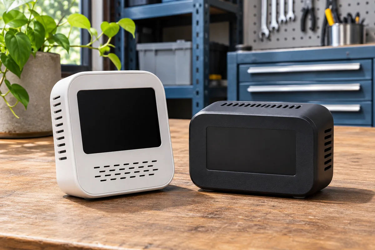
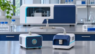
Compare instruments in the same air before using their difference to interpret a room and an intake.
Give the subtraction its own uncertainty check
If an indoor sensor reads high by 40 ppm and an outdoor sensor reads low by 30 ppm, the calculated excess is high by 70 ppm. If both are high by the same amount, the common offset cancels at those readings. Cancellation should be demonstrated rather than assumed. Independent transmitters can have different drift and concentration dependence. An outdoor enclosure, temperature change or pressure difference can change performance compared with the same device in a room.
For a simple conservative illustration, suppose each of two sensors has a possible ±50 ppm contribution under the actual test conditions. Allowing the two errors to oppose one another gives a possible ±100 ppm contribution to the difference. This is a bound for that example, without a probability or confidence statement. It excludes additional uncertainty from location, response time, averaging and assumed generation. Read each specification on its stated basis before combining limits.
For the six-person example, a nominal difference of 600 ppm becomes 500 to 700 ppm under that selected bound. Holding generation fixed, the inferred exchange spans about 39 to 54 L/s after rounding. The interval is asymmetric because flow depends on the reciprocal of concentration difference. At a much smaller difference, such as a nominal 100 ppm with a comparable error allowance, the denominator may approach zero. The resulting estimate can be too sensitive for a decision even if the air itself is well mixed.
To evaluate each device on the correct basis before taking a difference, see how to interpret a CO₂ monitor accuracy specification.
Berkeley Lab's commercial-building DCV monitoring research examined field sensor accuracy and selected systems that measured several locations through a common instrument. Some paired differences showed smaller errors than the absolute readings. That observation demonstrates a possible benefit of common instrumentation. It depends on shared error behavior and suitable sampling, with transport delay, leakage and carryover still worth checking.
Deal with near-zero and negative differences
At true steady state under the simplified model, a nonnegative indoor source produces a nonnegative difference. A negative observation should prompt a check of assumptions. An outdoor spike can arrive at the reference before it appears in the room. Indoor and outdoor clocks may be misaligned. An outdoor monitor may be sampling an exhaust plume that does not enter the room. A sensor offset can account for small apparent reversals. These possibilities call for different follow-up measurements.
If the indoor room begins below a changing outdoor background, the difference can briefly be negative during a physically reasonable transient. The steady-state inversion is invalid in that interval. Keep the observation in the data record along with its flags. Removing it solely because it disagrees with expectations can hide an outdoor reference problem.
A small positive excess can also have several meanings. A lightly occupied space may emit little CO₂. A space can have high outdoor exchange, or a local supply current may dilute the indoor sampling point. In a nearly empty space there may be too little signal to use occupant generation as a tracer. The useful response is to compare against the full operating context or use an independent method, rather than divide by a poorly determined number.

The one-zone calculation treats the room as one mixed volume. Multiple air streams or uneven concentrations call for additional evidence.
Keep the measurement record tied to a decision
Begin with the observation and label the next inference separately. A practical record includes the time window, indoor and outdoor locations, instrument IDs, averaging and quality flags, occupancy and activity, outdoor air mode, relevant doors and windows, and whether the concentrations were changing. It also records which differences are plausible given the uncertainty and which questions remain open. If the same investigation later relies on a new ventilation design, the preserved record allows the comparison to be reconstructed.
| Level of evidence | Useful result | Conditions to document |
|---|---|---|
| Time-aligned paired observation | The indoor sample was a stated number of ppm above the incoming reference | Sample locations, times, units, instrument checks |
| Comparison of repeat periods | Excess changed under a documented occupancy and operating context | Comparable instrument response, source activity and room state |
| Forward model comparison | Observed rise is broadly consistent or inconsistent with a specified airflow and source | Starting concentration, source, room volume, outdoor concentration and airflow assumptions |
| Conditional airflow estimate | A bounded one-zone exchange estimate for a near-steady period | Source magnitude, mixing, air paths, equilibrium and measurement error |
| Mechanical ventilation acceptance | Outdoor airflow or delivery meets the project method and criterion under tested modes | Appropriate independent measurements, equipment boundaries, system state and governing criteria |
For a room served by a variable system, plot the outdoor concentration and indoor concentration individually before plotting their difference. A change in difference can otherwise be misread as an indoor trend. Add known HVAC modes and occupancy events. If the controller changes airflow during the period, summarize how long each mode lasts. Avoid combining an intake baseline from one mode with indoor data from another mode.
Consider a room assessment with 520 ppm outdoors and 1,110 ppm indoors during a crowded hour. That is an observed 590 ppm excess. The same room gives an apparent excess of 710 ppm if an earlier 400 ppm background is used. A good record shows both the actual paired result and any comparison scenario that uses a fixed assumption. The specific flow question comes after reviewing whether the occupants and airflow remained stable long enough, and whether the sampled air represents the occupied volume.
When another method is needed
Use the CO₂ difference to target the next measurement. If the question concerns whether an outdoor damper meets a specified flow, measure outdoor air at the relevant equipment boundary using the applicable procedure. If the question concerns room distribution or interzone exchange, use additional sampling or a suitable tracer method. If the question concerns particles, odors or an indoor source other than human respiration, use measurements that address those hazards or emissions directly.
Itu Dokumen posisi CO₂ dalam ruangan ASHRAE Dan ASTM D6245 public scope explain why a single CO₂ number does not describe ventilation and overall indoor air quality in every space. An indoor–outdoor difference is more interpretable than a lone indoor reading when its reference and assumptions are documented. A mass-balance result still describes the boundary and conditions selected for the analysis.
Decide which part of the time series supports the comparison
A practical analysis can begin with a table of candidate intervals. For each interval, summarize the source activity, outdoor reference variability, sample validity, HVAC mode and whether the indoor value still has a sustained slope. Choose the analysis window based on the assumptions before looking for agreement with a desired number. If no candidate satisfies the conditions for inversion, report the observed differences and use the data to select a better measurement.
For example, consider a steady indoor concentration during an hour when people continue to enter and the outdoor-air damper opens in response. A stable value could reflect increasing generation balanced by increasing outdoor flow. A second hour might show the same average concentration with fixed occupancy and flow. The two windows have the same mean while carrying different evidence about steady operation. Review time-aligned occupancy and mode rather than treating low variability in concentration as proof that all model inputs were constant.
Outdoor variation also requires attention. When the incoming reference rises suddenly, the room responds over a mixing and air-exchange timescale. Subtracting the latest outdoor reading gives the concurrent difference at the sample points, which is useful to record. Treating that subtraction as a steady-state quantity immediately after the rise ignores the room's earlier background and accumulation. If a forward model includes varying outdoor concentration, use the measured input time series and state the model resolution.
Record concentration basis and units
Instrument outputs often use the convenient display abbreviation ppm. Confirm that the two points represent carbon dioxide on the same basis and use the same effective scaling. A controller could report an analog range conversion while a portable instrument displays its own compensated measurement. Verify documented environmental compensation and any correction applied upstream. A meaningful subtraction starts with comparable quantities and a clear record of how each value was obtained.
Similarly, keep the units of G and Q paired. If generation is entered in liters of CO₂ per second, express ventilation in liters of air per second before converting to another unit. An airflow calculated in cubic meters per hour cannot be compared directly with a design in liters per second. For a report, carry full precision through the arithmetic, then round the presented result to reflect uncertainty in generation and concentration.
Interpret a trend comparison between different room uses
Imagine two sessions with nearly equal occupancy counts and ventilation operation. The first is mostly seated work. The second alternates talking and movement. An observed rise in excess during the second session can reflect a larger source term even if the outdoor flow is unchanged. A repeat study can use a more detailed activity log, compare the same activity on different days, or use independent airflow evidence. That choice depends on whether the question concerns activity, ventilation performance, or both.
If the question is simply whether conditions changed after a maintenance action, a repeated comparison under similar use can be useful even without an absolute generation estimate. Name the observation precisely. For example, describe a lower occupied indoor–outdoor difference after the change during comparable sessions. This supports a narrower conclusion than a claimed increase in measured outdoor air.
Pertanyaan yang sering diajukan
Is 600 or 700 ppm above outdoors a universal target?
Those values can appear in specific guidance or examples. The relationship depends on occupant generation, room use, ventilation requirements and the relevant edition or method. Use the governing criterion for a project and treat a generic example as conditional.
Can I measure outside after the room test and subtract that value?
A later sample can help describe background if it is stable and comes from the relevant incoming air. A synchronized sample is stronger evidence. Local emissions, wind and changes in the active intake can make the later value unrepresentative of the earlier indoor interval.
Can I calculate air changes per hour directly from the difference?
The steady-state difference yields an exchange flow only when generation and the model assumptions are available. Divide that flow by the defined room volume in compatible time units to obtain an air-change estimate. The resulting value describes the exchange represented by the model.
Does a low excess establish that a room is healthy?
It can be consistent with low occupant emissions relative to air exchange during the observation. It leaves other contaminant sources, particle filtration and uneven air distribution to separate evaluation.
What if the room has two independent outdoor air paths?
Identify both paths and their concentrations. If incoming concentrations are essentially equal, the simple model may represent their total exchange under the remaining assumptions. If the concentrations differ or one path carries transfer air, use a balance that accounts for the individual terms or use a more direct measurement.






Tinggalkan Balasan