
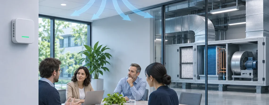
A CO₂ sensor's response time describes how its output approaches a new value after a defined change at the sensor. A ventilation control response also includes when the installed sensor encounters the change, when the controller can act, when outdoor airflow actually changes, and when that airflow affects the occupied zone. A sensor with a short T90 can be part of a system that takes much longer to change room concentration. To find the delay, record each transition on the same time axis and identify the first link where the expected change fails to appear.

A wall reading, the air handler and the occupied room represent different stages of the same response.
Identify the six clocks before timing anything
A person joins a meeting, a controller increases a ventilation request, and the room trend eventually levels off. It is tempting to subtract the timestamp of the first event from the last and call the difference sensor lag. That interval actually begins with a change in CO₂ generation and ends with a condition created by generation, incoming air, circulation and measurement. It includes several separate events that can overlap.
Start by writing the question as a pair of observable endpoints. A measurement technician might ask how long the transmitter takes to reach a specified fraction of a known input change. A controls engineer might ask how long it takes a valid point to produce an effective demand. A building operator might want to know whether a ventilation change improves the occupied room before a scheduled meeting ends. Each question requires its own reference signal and end condition.
| Timing layer | Start event | End evidence | Common reason for delay |
|---|---|---|---|
| Exposure and sampling | Local concentration changes or sample is switched | Change reaches sensing chamber | Room location, enclosure exchange, tubing or low sample flow |
| Đo đạc | Input step reaches sensing chamber | Sensor output reaches the specified fraction | Physical response, internal compensation or averaging |
| Acquisition and logging | Sensor reports a usable value | Controller or historian records it | Polling interval, scheduling, clock mismatch or history compression |
| Control logic | Valid measurement satisfies defined conditions | Effective control request changes | Filtering, persistence, mode gate or priority |
| Mechanical delivery | Effective request changes | Required actuator position and airflow are verified | Actuator travel, fan ramp, damper fault or static pressure |
| Occupied-zone response | Actual delivered airflow or generation changes | Local room concentration follows an interpretable trend | Air replacement, redistribution, continuing emissions or changing occupancy |
A clock can be absent or effectively instantaneous for a given setup. A hardwired input has no network polling across that segment, but the controller can still scan and filter it. A command can be generated promptly while a minimum run timer elsewhere limits when it takes effect. An historian can show stale information while the local loop continues to use fresh samples. Treat the table as an evidence map and use only the layers that apply.
Read the response specification under its stated test conditions
For a step from 500 ppm to 1,000 ppm, the output reaches 90% of the change at 950 ppm, assuming it started at 500 ppm and eventually stabilizes at 1,000 ppm. For a falling step from 1,000 to 500 ppm, the 90% point is 550 ppm. T90 is measured from the defined start of the input event to the output crossing that fraction. The input step definition, observed output, starting value and terminal value matter as much as the time written in the data sheet.
A measured T90 may include part of the test fixture or signal processing depending on the documented method. Check whether the value describes a bare module, a powered transmitter in its enclosure, a forced-flow path or a diffusion arrangement. Confirm which sample mode applies, whether the device is warmed up, and whether the response figure is typical or guaranteed. Compare upward and downward behavior only when both have been established. A filter or inlet arrangement can introduce behavior the manufacturer never tested with the module.
The Senseair eSENSE FAI specification for article 050-8-0061 lists T90 below 10 seconds at 30 cc/min and a diffusion time below 3 minutes. Those figures belong to the configurations identified in the specification. They do not establish the time for a wall transmitter to see the average of a real meeting room. Senseair eSENSE FAI specifications
Sensirion lists 60 seconds at the 63% response point for the SCD43 CO₂ module. For an ideal first-order response, the fraction completed at time t is 1 − exp(−t/τ), so 63.2% occurs at one time constant and 90% at ln(10) × τ, approximately 2.303 × τ. A 60-second time constant would therefore imply about 138 seconds to 90% in that model. That is arithmetic for an assumed response shape. It is not a published SCD43 T90 or a substitute for data from the assembled product. A pure transport delay, multiple thermal or exchange processes, nonlinear filters and discrete reporting can all make the conversion unreliable. Sensirion SCD43 specifications
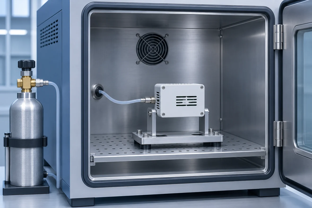
A fixture test defines the input event and the output under observation. Installed exposure adds its own conditions.
Calculate the scale of a room response
A room can begin responding to a change in ventilation before its CO₂ concentration changes enough to stand out on a plot. For an idealized well-mixed single zone of volume V, with outdoor airflow Q, steady outdoor concentration Cₒ and no indoor generation after occupants leave, excess concentration follows:
C(t) − Cₒ = [C(0) − Cₒ] × exp[−(Q/V)t]
Use consistent units. If Q is expressed in cubic meters per hour and V in cubic meters, Q/V is in inverse hours and t is in hours. The result assumes that the incoming air has the stated outdoor concentration, that Q is steady, that air leaving has the concentration of the mixed room, and that the comparison instrument tracks that concentration well enough. A separate air exchange path with a different incoming concentration needs a different model.
For a hypothetical 240 m³ room receiving 480 m³/h of outdoor air, Q/V is 2 h⁻¹. The room time constant V/Q is 30 minutes. If the room starts at 1,220 ppm and outdoor air is 420 ppm, the initial excess is 800 ppm. After 15 minutes the excess is 800 × exp(−0.5), or about 485 ppm, giving about 905 ppm indoors. After 30 minutes it is about 294 ppm, giving about 714 ppm indoors. It takes about 69 minutes to remove 90% of the initial excess, at which point the idealized room would read about 500 ppm. Those values illustrate the model at a chosen airflow and carry no acceptance significance.
| Elapsed time from the modeled change | Modeled indoor CO₂ | Fraction of initial excess remaining |
|---|---|---|
| 0 min | 1,220 ppm | 100% |
| 15 min | 905 ppm | 61% |
| 30 min | 714 ppm | 37% |
| 60 min | 528 ppm | 14% |
| About 69 min | 500 trang/phút | 10% |
With continuing generation, concentration approaches a different endpoint. In the same idealized model a constant volumetric CO₂ generation rate G, expressed on the same volume and gas basis, gives a steady excess fraction G/Q. The trajectory can rise after the damper opens if the new steady concentration is still above the current concentration. The slope may become less positive while occupants continue to exhale CO₂. Opening a ventilation path does not make people stop generating CO₂, so a successful delivery event need not coincide with an immediate declining trend.
NIST's Indoor Carbon Dioxide Metric Analysis Tool estimates a time-dependent concentration from space characteristics, people and outdoor ventilation rather than a universal concentration. ASHRAE's ventilation handbook also discusses imperfect distribution and the distinction between supplying air and delivering it effectively. In a real building, a single wall point can see a nearby plume, short-circuiting airflow or cross-zone transfer. A fitted decay from one point therefore needs the mixing, occupancy and airflow assumptions to be established before it is used to estimate ventilation. NIST Technical Note 2213, ASHRAE Handbook chapter on ventilation and infiltration

Supply air travels through an occupied space before a wall point sees a representative change. Air paths are illustrative.
Trace the signal before changing the control tuning
Compare the local transmitter output, raw BAS input, filtered value used by the sequence and historian export. A discrepancy between local and raw BAS values points toward scaling, communication, polling or source selection. Agreement at that boundary with a delayed filtered point points toward signal conditioning. If both raw and filtered points meet the trigger but the request stays fixed, inspect occupancy mode, threshold persistence, enable logic and priority. These are separate tests even when the same software supplies all four values.
A moving average adds different apparent lag depending on the disturbance. After an ideal step, a trailing average of duration W that was filled with the old value ramps to the new level over W. It reaches 90% after approximately 0.9 W in a continuous model. A 2-minute window can therefore create an approximately 108-second 90% response to an instantaneous step before any extra delay from sensor dynamics or controller timing. A real rolling average can operate on discrete samples, skip invalid values or behave differently after reboot. A threshold crossing also depends on the size and initial level of the disturbance, so this calculation gives the scale of an effect without predicting a complete sequence.
Persistence is different. If a sequence requires the filtered point to stay above a threshold for two minutes, the timer begins only after the filtered point crosses and may reset when it drops below. A demand can therefore fail to assert during a brief real spike even though the transmitter recorded it correctly. A short event can also disappear in a coarse historical record while the controller acted on every local scan. Check the interval and timestamp source for both the live decision and the trend used to reconstruct it.
In a networked system, periodic acquisition adds phase-dependent waiting. If a gateway reads a changing point every 30 seconds, and readings arrive on time, the next poll could occur just after the event or almost 30 seconds later. Delays on a busy field network, skipped updates and retries complicate that range. If a historian then samples on a separate clock, its newest record may lag by another interval. Compare event timing at the source and receiver before declaring that the controller responded when the plotted line moved.
Verify the command, the motion and the airflow
A damper command identifies the requested state, and a position feedback signal identifies the state reported by its sensor or actuator. Neither alone establishes outdoor airflow. Blade linkage may be loose, fan speed can vary, system static pressure can change and a competing sequence can alter the effective command. The same blade angle can yield different intake flow under different pressure conditions. Identify the measurement used to confirm airflow and the operating range over which it is valid.
An outdoor-air measurement at an air handler establishes delivery at that measurement boundary. In a multizone system it leaves a second question about distribution to the relevant space. Primary zone airflow, outdoor fraction, occupancy diversity and transfer paths can all matter. A zone terminal may supply more recirculated mixed air while the outdoor intake stays almost unchanged. Conversely, a central intake change may produce different room responses across a building because zone demand and air distribution differ.
When inspecting a step event, separate the requested command from the one that wins arbitration, then identify the first observed change in fan proof, position and airflow. Check any project limits and hand-off between supervisory and local loops. A sudden raw CO₂ change with no fan proof deserves a different investigation from airflow at the air handler with no observable change at a wall point. ASHRAE Handbook chapter on controls design and application
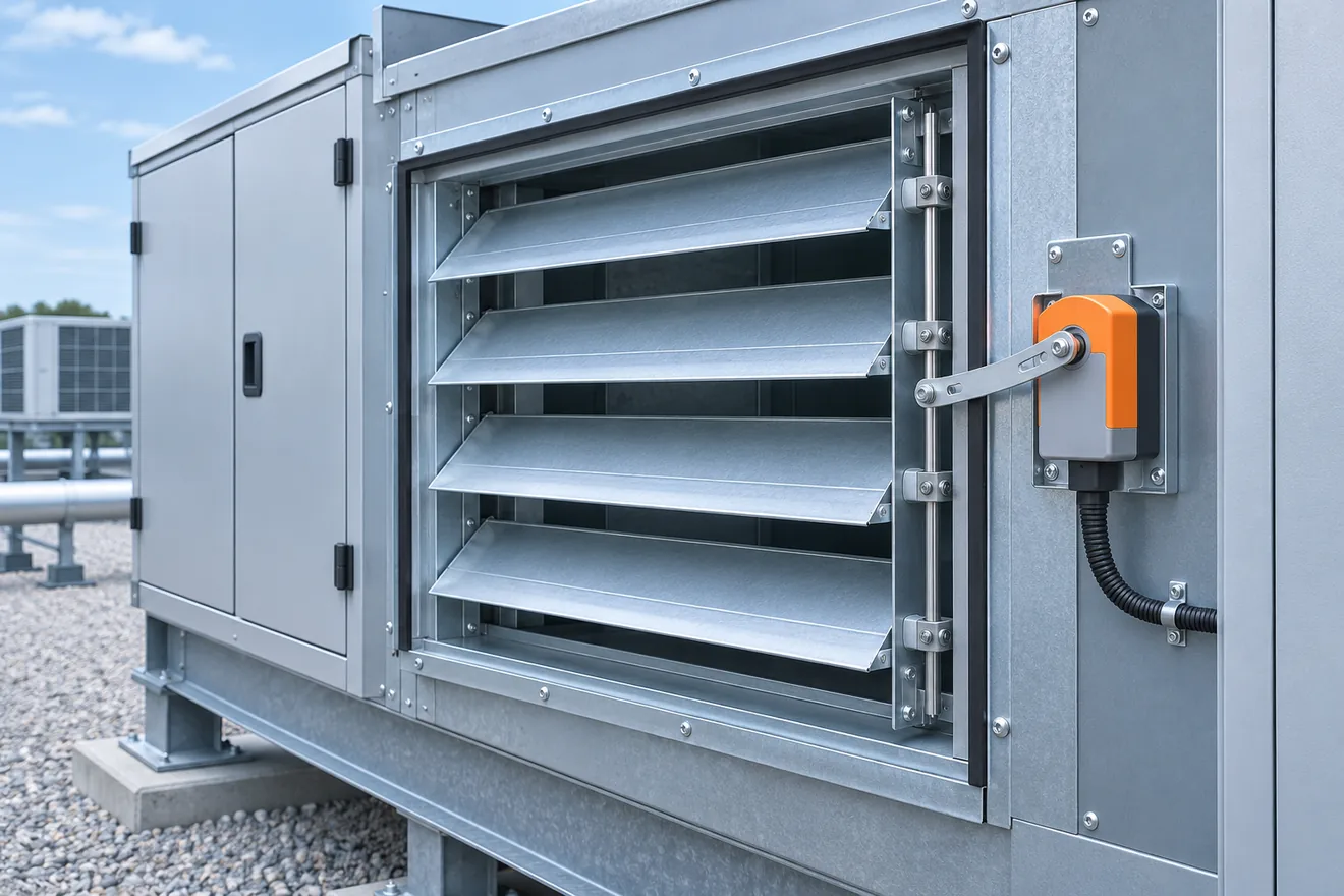
Command, motion and outdoor-air delivery can each be verified at a different boundary.
Work through an aligned event
Consider a hypothetical single-zone office test with clocks checked against a common reference. The site has a direct CO₂ point, a filtered point, a demand point, damper feedback, fan status and valid outdoor airflow measurement. The procedure records the mode before the event and keeps it stable long enough to interpret the result. At 09:00 the occupancy count begins to rise. At 09:03 the raw transmitter value starts increasing and the gateway records the change. The filtered point reaches the project's test condition at 09:05. At 09:07 the controller asserts demand when its configured persistence expires. By 09:08 the actuator reports movement, and at 09:09 the airflow measurement confirms increased outdoor flow. The room trend continues rising until 09:13, then levels off as occupants and HVAC mode remain stable.
The three minutes after occupancy begins do not measure transmitter T90. The concentration change at the sensor inlet was neither observed nor a defined step. The two minutes from criterion crossing to demand are consistent with the configured persistence. The two minutes from demand to proved airflow include mechanical and delivery behavior. The remaining room trend reflects ventilation, generation, distribution and measurement. The series can support further investigation but cannot isolate a sensor time constant without a defined input test.
For a counterexample, suppose the same room's damper command changes but airflow stays within measurement uncertainty and fan status remains normal. Stop interpreting the CO₂ curve as proof of a ventilation response. Review the air path, damper feedback, effective command and reliability of the airflow measurement. If the airflow instrument is out of its valid low-flow range, the trace cannot distinguish small flow from instrument limitations. Record that gap and obtain the measurement required by the project before assigning a cause.
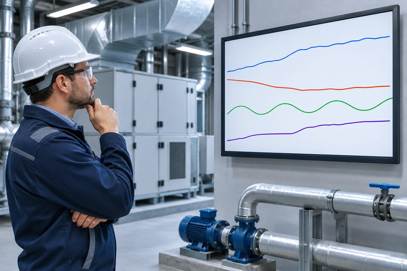
Synchronized evidence makes the order of transitions visible. The traces are conceptual.
Design a comparison that can distinguish a delay from a display artifact
Decide which boundary the test addresses before collecting data. For a measurement comparison, select a compatible independent instrument with suitable range, known response and documented condition. Position both instruments to observe comparable air without directing someone’s breath into the inlets. Record instrument warm-up, sample path, output averaging and timestamps. When a manufacturer-approved fixture step is appropriate, record the delivery method and reference signal used to confirm the step. A person exhaling beside a wall sensor creates a poorly defined plume and is unsuitable for estimating T90.
For a sequence review, retain sufficient resolution around the expected change. A one-minute history can show the order of events separated by several minutes but may never distinguish a 15-second actuator event from a 30-second acquisition delay. Select a permissible interval with adequate separation, check device and historian clocks, and record whether displayed points use event timestamps or receipt timestamps. Save the unaggregated export so later analysis can distinguish a flat line from a change-of-value archive that omitted repeated readings.
Record the names and units of measurements, commanded and proved positions, fan state, valid outdoor and zone airflow when available, zone occupancy context, system mode and any override. For verification involving a real HVAC sequence, use the approved project procedure and restore the agreed normal mode. A demonstration under a temporary mode should carry that label through screenshots, raw exports and the signed test record. A matching graphic from normal operation does not by itself prove that the same logic was exercised.
Use repeated observations when normal occupancy varies. Two events can have the same maximum CO₂ and very different times to peak because the occupants entered at different rates or ventilation was available earlier in one case. Compare the event sequence rather than treating the peaks as equivalent input steps. The practical goal is to find a timing change supported by independent observations. Độ ẩm ảnh hưởng đến kết quả cảm biến khí như thế nào covers a separate class of measurement changes that can complicate field comparisons.
What does the evidence let you rule in?
Timing investigations often produce two records that look inconsistent at first. A handheld reading may change within seconds while a BAS graph is flat, or a controller may show an earlier command than the export can display. Before adjusting equipment, compare measurements with the same intended meaning. A portable device in a person's breathing plume and a fixed sensor at a representative room site are observing different local air. A trend sampled on a minute boundary and a controller event recorded when the logic ran are observing different timestamps.
| Aligned finding | Where the evidence narrows the problem | What is still open |
|---|---|---|
| Local reference changes, transmitter output changes later | Exposure, sensor response or transmitter filtering | Whether the two inlets saw the same input |
| Local output changes promptly, raw BAS point updates later | Acquisition, gateway mapping or timestamps | Whether the controller uses the trended point |
| Raw and filtered values cross at different times | Controller input conditioning | Whether the filter is operating as designed |
| Effective request changes without position proof | Mechanical response or proof point | Whether the actuator actually moved |
| Proved position changes without measured flow change | Delivery, pressure or flow measurement | Whether the method resolves that operating range |
| Proved flow changes before a clear room trend | Zone dynamics, continuing generation or measurement | Which rooms and locations received the change |
When the next action depends on a short delay, define what a change means. A crossing of the new value can be caused by noise or overshoot. An endpoint that requires the signal to remain within a band for a specified period answers a different question from first crossing. A chart whose scale rounds to the nearest 50 ppm may mask an earlier shift seen in an unrounded export. Document whether the comparison uses first detectable change, a threshold crossing, a specified fraction of a step, or a maintained final condition.
A second comparison can deliberately isolate the time layer of interest. A comparison in stable, well-represented room air can test agreement and identify unexpected jumps. It cannot determine a step response because the input lacks a known transition. An authorized controller input simulation can test the persistence, arbitration and command boundary. It bypasses sensor exposure and measurement. A documented airflow response test can verify delivery under its operating conditions. It cannot attribute a room concentration change to outdoor airflow when occupancy or adjacent transfer air changed at the same time. Combine these records when the question spans several layers.
When a faster sensor would help
A faster sensor helps when the measurement channel accounts for enough delay to affect the intended decision and the installed exposure allows the change to reach it. For example, if a defined fixture step reaches the transmitter inlet quickly, the raw output is consistently late under the relevant mode, and the controller acts promptly once the new value arrives, the installed transmitter merits attention. Check whether its enclosure, inlet, flow condition or selectable output processing explains the measured behavior before treating a module specification as the solution.
A shorter acquisition interval helps when the raw sensor value becomes available quickly but the receiving point misses or delays it. It has little effect when the dominant delay is air exchange in the zone, or when the existing network cannot reliably sustain the added reads. A shorter persistence period changes the logic, which can make the sequence more responsive to both meaningful occupancy and brief local plumes. Evaluate the intended control stability and approved change process before revising that setting.
A mechanically verified airflow increase may still leave an undesirable occupied-zone pattern. Check the real air distribution, outdoor fraction, mixing and time occupied before replacing the measurement hardware. A room with furniture or partitions added after balancing can deliver differently at the observed site. Conversely, if multiple suitable locations show similarly slow dilution and outdoor airflow was independently verified, the physical timescale may simply be consistent with the room volume and flow. Compare the measured trajectory and its uncertainty against the applicable design question, using the single-zone model only where its assumptions are reasonable.
Câu hỏi thường gặp
Does a 30-second T90 mean ventilation responds in 30 seconds?
It describes a defined sensor response under specified conditions. Airflow response requires evidence of actual delivery, and the occupied-zone concentration has its own dynamics after delivery. Define which interval you need to verify before using the specification.
Can two T90 values be added to estimate system response?
Separate pure waiting times can be added when their endpoints and ordering are known. The 90% times of two cascaded dynamic responses do not generally add to the combined 90% time. Their output shapes and delays matter. An end-to-end test with a defined input and observed output establishes the timing for the tested conditions.
Why can CO₂ rise after a working damper opens?
People continue to generate CO₂, and the new outdoor airflow can be insufficient to make concentration immediately decrease from its current value even though it reduces the rate of increase. Distribution, occupancy timing and averaging also affect the observed slope. Compare proved airflow, occupancy and the trajectory over a suitable interval.
How do I distinguish controller lag from historian lag?
Compare a timestamped local sequence or command event with the raw point, filtered point and stored trend. Verify clock alignment, receipt versus event timestamps and logging policy first. A historian interval can conceal a fast event that the controller used correctly.
What can one room sensor establish about air mixing?
It establishes the concentration history near its sensing location within the limits of the instrument. A representative zone interpretation needs a justified location and, where uncertainty matters, comparison at other positions and under relevant operating conditions. A mathematically smooth decay does not prove that the room was well mixed.





Để lại một câu trả lời