
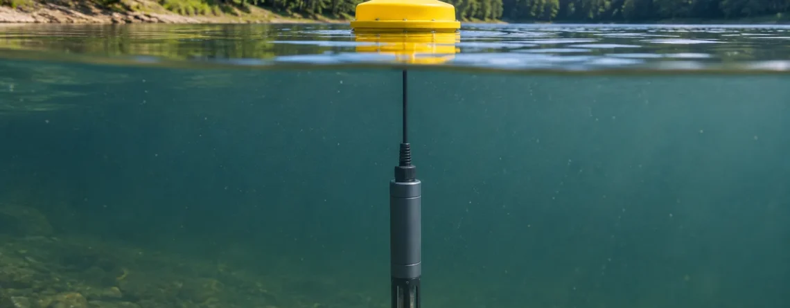
A chlorophyll fluorescence sensor shines light into a small volume of water and measures the red light emitted by pigments in suspended algae and cyanobacteria. The response is an optical proxy. With stable conditions it can show when pigment-bearing particles increase or decrease at the sensor. Paired water samples can establish how well the response estimates chlorophyll a concentration at a particular site. The strength of that relationship depends on the water, the organisms, and the light they have been exposed to.
A station can record a clear drop in fluorescence at midday even when a laboratory sample shows nearly the same chlorophyll a concentration as it did in the morning. A different station may see its fluorescence fall because the probe slipped below an algae-rich layer. The curves can look similar, but the checks are different. In the first case you compare readings against light exposure and extracted pigment. In the second you confirm depth and measure above and below the probe.
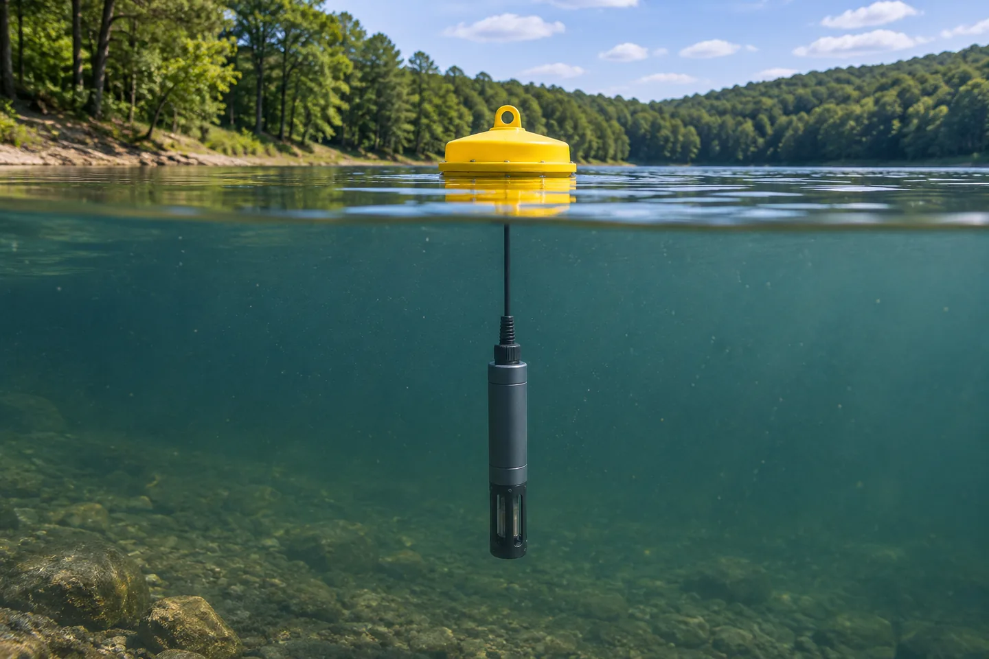
An immersed probe measures the water around its optical head. A buoy record can describe conditions at one depth while the reservoir varies vertically and horizontally.
What the sensor actually measures
A field fluorometer has a light source, typically an LED, and a detector behind an optical filter. The LED sends excitation light through a window into the water. Chlorophyll absorbs some of that light. A small share of the absorbed energy comes back as fluorescence at longer wavelengths, in the red part of the spectrum. The detector receives a fraction of that emission. The optical design helps separate it from reflected excitation light and other light reaching the instrument.
A blue excitation band and a red emission band are common for this measurement. USGS lists one EXO configuration at 470 nm excitation and 685 nm emission and a Wetstar configuration at 460 nm excitation and 695 nm emission. Those are examples from particular instruments. Differences in bandpass, geometry, gain, and calibration can change the relative response, particularly when instruments encounter a changing mixture of organisms. See USGS field techniques for algal pigment fluorescence, table 3。
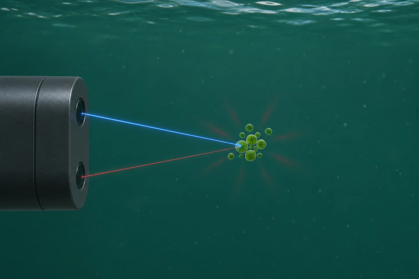
Blue light excites pigment in the water. The red path shows the small share of emission collected by the detector. The drawing simplifies the optical geometry and the volume of water sampled.
The instrument commonly reports counts, relative fluorescence units (RFU), or a reading scaled as chlorophyll in micrograms per liter (µg/L). Counts and RFU are instrument response measures. Check the manual for the scale, averaging and gain conventions. A value of 20 RFU on one model may correspond to a different optical response on another. Even replacement sensors of the same model merit an overlap check before you join their records.
A fluorometer can also display a concentration equivalent using a factory or user calibration. Its units look like the units on a laboratory report, but the quantities are obtained in different ways. The probe observes intact particles and cells in water. The laboratory measures pigment recovered from a known volume using a specified analytical method. A documented comparison can show whether the sensor's concentration scale is accurate enough under field conditions. The Turner Designs AquaFluor manual describes these as separate operating modes and discusses comparing an in-water response with extracted chlorophyll.
Chlorophyll, biomass, species and toxins answer different questions
Chlorophyll a concentration is the mass of that pigment per volume of water. Algal biomass refers to the amount of algal material. Programs may report related quantities such as cell biovolume, cell abundance, or mass estimated using a defined method. Chlorophyll a is often used as an indicator of phytoplankton biomass because photosynthetic organisms contain the pigment. The amount per cell or per unit biomass can shift with organism type and growth conditions. Even a laboratory chlorophyll result therefore needs ecological context when you interpret it as biomass.
Some sondes add a channel for phycocyanin (PC) or phycoerythrin (PE). These accessory pigments can improve screening for particular groups when the instrument and local community support the comparison. A phycocyanin channel is often useful for freshwater cyanobacteria screening. Its response also varies with organisms, optical interference, and physiological conditions. A rise on that channel can justify collecting a sample for identification. A channel ratio can also change when light and community composition affect the two signals differently, so interpret it within a locally tested use.
| Monitoring question | Measurement to use | How a field fluorometer can help |
|---|---|---|
| When did the local pigment signal change? | Quality-controlled RFU or counts from a documented setup | Continuous records can show when a change started and when to collect a sample. |
| How many micrograms per liter of chlorophyll a were present? | Extracted chlorophyll a by a defined lab method, or a validated site-specific estimate | A tested relationship can extend the laboratory record between paired visits. |
| How much algal material or how many cells were present? | A biomass, biovolume or cell-count method matched to the question | Chlorophyll can act as a relative biomass indicator where pigment content and composition are sufficiently stable. |
| What organisms are present? | Microscopy or an appropriate taxonomic or molecular method | Accessory pigment changes can help prioritize a sample for identification. |
| Which toxins are present and at what concentration? | Toxin-specific analysis using a method appropriate to the water and analytes | An optical change may prompt a sample. The toxin concentration comes from the toxin method. |
For example, EPA Method 546 measures total microcystins and nodularins in drinking and ambient waters. Different analytes can require different assays. For a recreational or drinking-water program, follow the program's sampling and decision procedure for toxin questions. A station's chlorophyll trace is valuable for finding times to investigate. See EPA harmful algal bloom methods。
Why the signal changes when pigment concentration stays steady
Think about three parts of the measurement. First, the amount of pigment in the water sampled by the probe can change. Second, the same amount of pigment can emit a different amount of red light. Third, a different fraction of the light can reach the cells or return to the detector. Start with those possibilities when you see a change, then look for independent evidence.
Bright light and nonphotochemical quenching
Under strong light, photosynthetic organisms can dissipate more absorbed energy as heat. The fluorescence yield can fall, which means the probe receives less red light per unit pigment. This process is called nonphotochemical quenching. The organisms' light exposure before the reading matters, so readings at similar light levels in the morning and afternoon can behave differently.
A controlled study exposed cultures of a green alga and a cyanobacterium to a simulated daily light cycle and observed suppression of pigment fluorescence across three commercial probes. The study also found that suppression could persist during declining light. The effect was measured under particular organism and light conditions. At a field station, a repeating midday dip and dusk rebound is a reason to compare with local light and extracted pigment. A correction from another site or instrument may erase genuine changes. See the original light-induced quenching study。
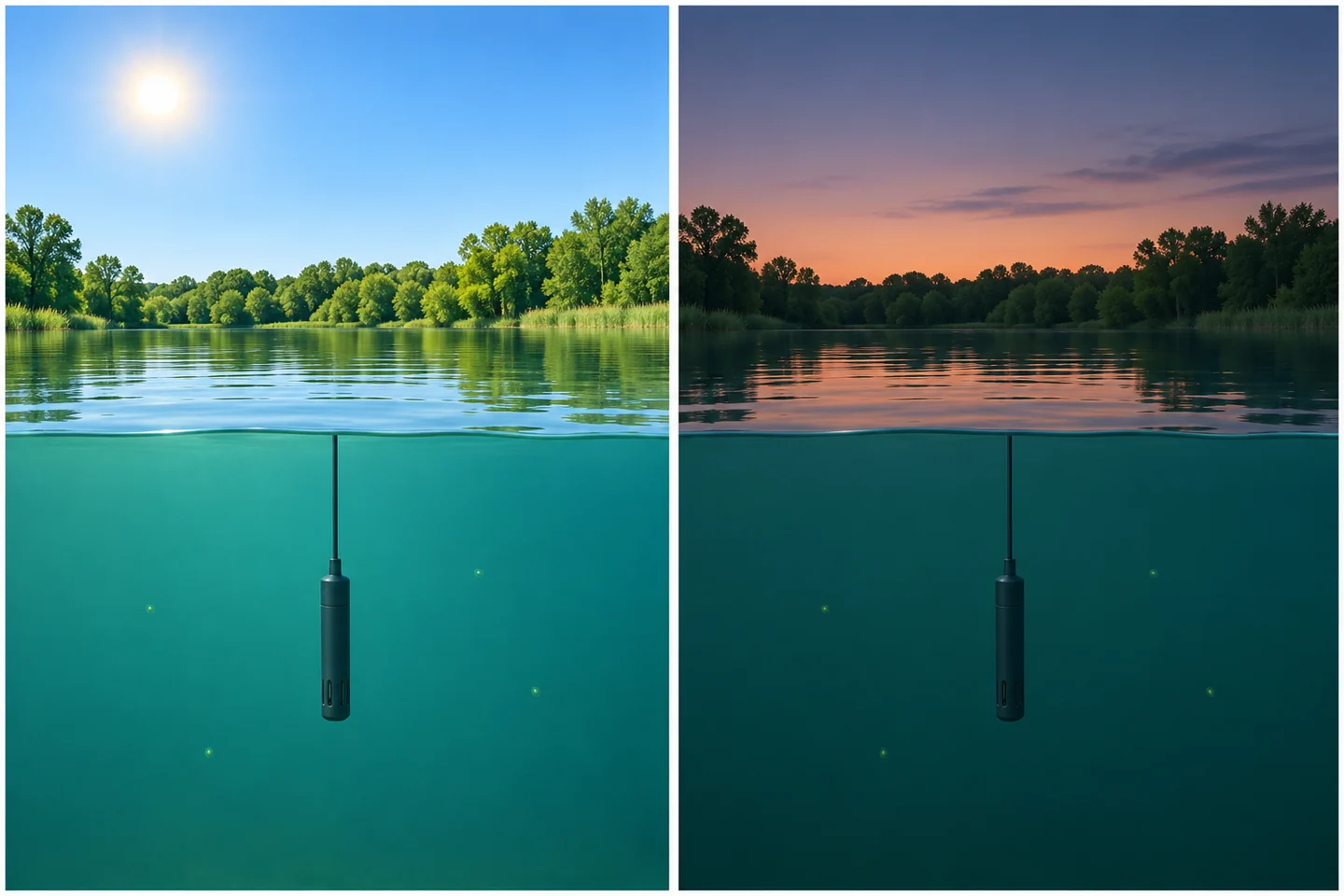
Light exposure can change fluorescence yield even when pigment abundance is steady. Changes in depth, mixing and cell distribution can also affect a real station's daily pattern.
For a fixed shallow station, log light or available indicators such as local solar conditions, time, cloud cover and depth. Compare matched laboratory samples across different light conditions if daytime estimates matter. For a profiler, compare the same depths where possible and remember that light and community composition may both change down the water column. A consistent after-dark window can improve comparability for some trend questions. It also selects a different period of the biological cycle, when buoyant organisms may have moved. Label the time window in any derived record.
Particles, color, bubbles and temperature
Suspended solids and colored dissolved material can absorb or scatter excitation light before it reaches pigments, or affect the emitted light before it reaches the detector. Depending on the instrument and the water, scatter or fluorescence from other substances can also contribute to the detected signal. During a runoff event, the sensor response may be altered even as flow carries a different algal population past the probe. A turbidity channel helps flag when that change in optical conditions occurred. To interpret its own units and measurement conditions, see how water turbidity sensors report NTU and FNU。
Bubbles can intermittently cover an optical window or change how light is scattered. Check for them downstream of aeration, near a pump inlet, or at a high point in a bypass. Temperature can affect the instrument's electronics and the fluorescence response of the sample through different mechanisms. Ask which of these the instrument compensates for. A correction built into a device may also have a defined operating range or be specific to a calibration standard. Keep the measured water temperature with the pigment record.
At the high end, a flat trace may mean the output reached its maximum, gain changed, or the detector response departed from linearity. At the low end, small shifts around the blank can be large relative to the signal of interest. Logging more decimals leaves that limitation intact. Record over-range flags and gain changes so that a later reviewer can distinguish a plausible plateau from a scale limit.
| Pattern in the record | 合理的解释 | Field check that narrows the cause |
|---|---|---|
| Midday dip and evening recovery on clear days | Quenching, vertical movement or changing water mass | Compare light, probe depth and extracted pigment across the pattern. Take a short depth profile where stratification is plausible. |
| Shift during runoff or resuspension | Attenuation, scattering, dissolved color or actual pigment transport | Check turbidity and water color, then collect a matched grab while the changed water is present. |
| Brief irregular jumps near pump cycling | Bubbles, flow-cell filling or a real transient slug | Match timestamps to pump and flow records. Inspect the cell and take a paired reading after flow stabilizes. |
| Slow drift followed by a step at service | Fouled optics, instrument drift, or a changed depth or orientation during service | Record as-found condition and positions. Compare before and after cleaning under stable conditions, then verify with a reference. |
| Repeated readings at the same upper limit | Clipping, a data logger limit, or genuine persistence | Compare raw output with the configured range and range flags. Use a suitable range or collect a lab sample for the event. |
| Gradual increase with clean optics and otherwise stable conditions | More pigment, higher fluorescence yield or a changing organism mixture | Collect same-depth pigment samples and, where composition matters, obtain cell or taxonomy observations. |
Install the probe where it sees the water you want to describe
Decide which water the record represents before selecting a mounting point. A probe just below the surface can serve as an early warning at that depth. A probe near an intake can answer what water is approaching the intake. A depth profile can find an algae-rich layer that a fixed station never sees. In each case the probe's small optical volume represents a larger area only to the extent that the water around it is representative.
For an immersed sonde, keep the optical head below the lowest expected water level and away from the bed, structures or reflective surfaces according to the manufacturer's clearance guidance. Note what the mounting depth is referenced to. A fixed probe attached to a pier can sit deeper below the surface after a rise in water level. A floating mount can maintain a nearly constant depth below the surface while moving relative to the bed or intake. In either arrangement document installation height and the actual depth when taking validation samples.
A bypass places the sensor in a flow cell for easier access. Check whether the intake samples the intended layer and whether the water arrives with bubbles, settled particles or retained material in the line. Maintain the manufacturer's flow and pressure conditions. Keep the flow path short enough for the intended time resolution and record changes in pump state. As a simple estimate, a line holding 2 L with a measured flow of 1 L/min has a nominal two-minute transit time. A sensor reading at 10:02 would then pair with water entering the intake at about 10:00. Mixing and additional cell volume can broaden or delay that response. A grab from a representative port near the sensor often simplifies the pairing if the question is what the sensor actually saw.
For selection, check the pigment channels, the option to export RFU, the expected range, the optical clearance and mounting restrictions, and how the instrument reports faults. Compare the value of a wiper, a more accessible mount, and a second reference sensor against the station's actual service schedule. A probe that remains clean only for the first few days of a monthly deployment leaves most of that record difficult to defend, regardless of its initial sensitivity.
Separate cleaning from calibration
Biofilm or sediment on a window changes the optical path. A film can shade the sample, scatter light, or contribute its own fluorescence. A wiper can help keep the optical area usable, but the wiper itself can wear, bind or carry debris. Establish an inspection interval using what the windows actually look like and how the readings behave across successive visits.
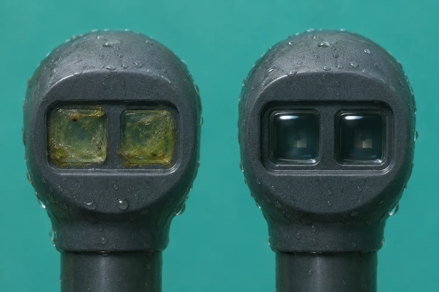
The window is part of the measurement path. A film can alter the reading before it looks thick enough to obscure the probe.
At a service visit, record the as-found time, depth, output and optical condition before moving or cleaning the probe. Clean using the procedures and materials approved for that instrument. Confirm wiper operation where fitted and return the head to its documented position. Once the reading settles, compare it with the as-found value. If the water changed during the visit or the probe came back at another depth, the difference includes those changes too. A large cleaning step is grounds to review the interval. It seldom tells you when the film started or exactly how it grew.
After cleaning, verify the instrument against the prescribed blank and suitable check reference. A blank tests baseline response under specified conditions. A stable dye or solid check reference, when supported by the manufacturer, tests sensitivity or repeatability in its prescribed setup. Note the reference lot or identifier and temperature if relevant. A standard can verify repeatable instrument response while the site relationship between RFU and chlorophyll remains uncertain. Use the check history to decide when recalibration is needed and save the pre-adjustment results alongside any changed settings. See USGS field maintenance and calibration guidance。
A useful distinction in the station log is fouling when material changed the optical path, drift when a clean sensor changed its response to a stable reference, and field bias when otherwise acceptable instrument readings systematically disagree with matched laboratory pigment data. The first two can occur together. A well-documented cleaning visit and an independent reference help separate them. Where you correct historical data, retain the original values, mark the edited interval and record the evidence behind the correction.
Validate concentration estimates with matched grab samples
A grab sample is a discrete sample of water. For a useful comparison it must represent what the fluorometer saw. Match horizontal position, depth and time. Keep the sampling device clear of the probe's windows and avoid stirring bottom sediment or introducing air at the optical head. A sample skimmed from the surface answers a different question from a fixed probe several meters down, even when both are from the same station.
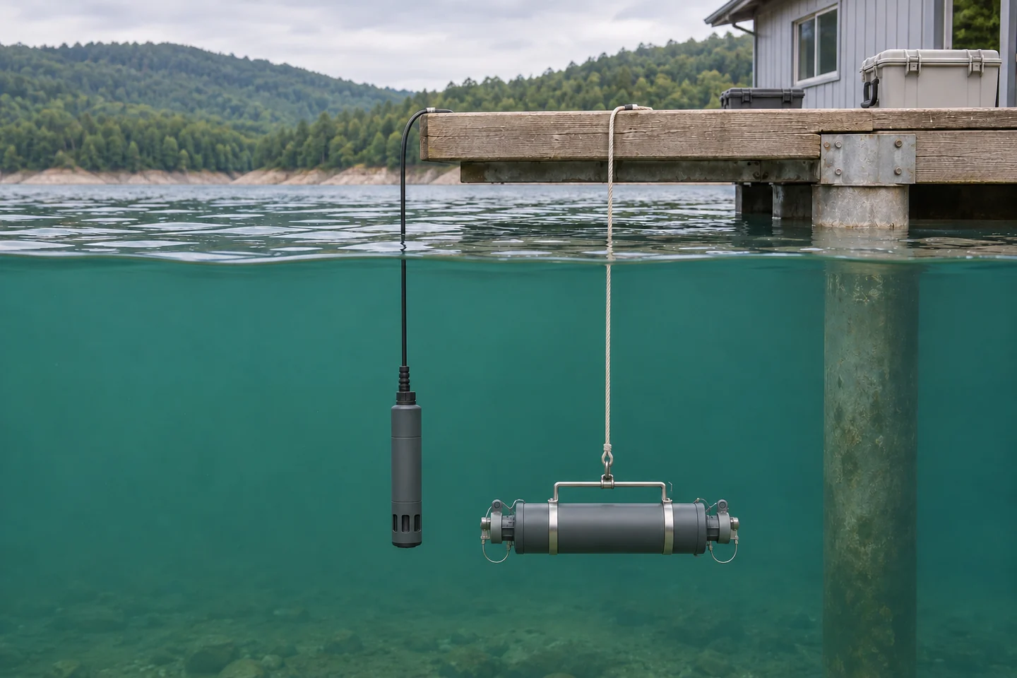
Pair the probe value with a sample from the water around the optical head. A distinct surface sample can be useful for a surface question and should be identified separately.
- Agree on the laboratory measurand. Ask the lab which chlorophyll method it reports, how it handles degradation pigments, and what filtration, containers and handling it requires. In EPA Method 445.0, pigment is collected by filtration, extracted and measured fluorometrically. Laboratory methods can differ in the treatment of compounds such as pheophytin a. Keep the method and reporting conventions stable across calibration and validation samples. See EPA Method 445.0。
- Capture a documented pair. Record sample ID, collection time and time zone, station, depth, raw signal, the instrument's reported units, and its configuration. Use an appropriate stable logging window around the grab and record that window. In a rapidly changing event, an hourly average can hide the signal that corresponds to a sample taken during a brief spike. Save temperature, turbidity, light or weather, instrument status and the last service date.
- Sample the range where the estimate will be used. Include baseline and elevated pigment levels. Sample the combinations of season, light and water conditions that could change the relationship. Several samples from one clear afternoon can improve repeatability estimates for that afternoon. Add independent visits to learn whether the relationship transfers to other days or a storm. Consider duplicate grabs when short-distance patchiness is likely.
- Fit and check separately. Plot extracted chlorophyll against fluorescence. A simple linear fit may be useful over a demonstrated range, provided its errors fit the decision. Examine errors by concentration, turbidity, time of day and season. Hold out visits or events so the same event does not dominate both fitting and checking. A high correlation can coexist with systematic low estimates in bright or colored water.
- Set an explicit reporting scope. Record the sensor, calibration version, site, validation range and environmental conditions. Flag values outside that scope. Compare an overlap period when you replace a sensor or change configuration. If the field relationship becomes unreliable during a different season or water condition, use the RFU as a qualified trend signal where it is still useful and continue reporting the independent lab results.
The continuous and discrete records serve different sampling needs. A sonde resolves changes between visits. A lab grab provides an independent measure at its collection time. An experimental comparison using freshwater mesocosms illustrates the amount of calibration and data review involved in deriving equivalent chlorophyll from in-water sensors. It also illustrates why results from a particular setup should travel with the setup and conditions that produced them. See the mesocosm comparison of sensor and laboratory chlorophyll。
Worked example of a fit that needs a condition flag
Suppose a hypothetical reservoir station fits estimated chlorophyll a in µg/L = 1.0 + 0.50 × RFU using earlier visits. The fit was built over 4 to 30 RFU. The equation would predict 10.0 µg/L at 18 RFU. Now compare two later visits, both within that signal range.
| Held-out visit and signal | Estimated chlorophyll a | Extracted chlorophyll a |
|---|---|---|
| Calm morning, 18 RFU | 10.0 µg/L | 9.0 µg/L |
| Clear afternoon, 10 RFU | 6.0 µg/L | 11.0 µg/L |
Subtract the laboratory results from the estimates. The morning residual is +1.0 µg/L and the afternoon residual is −5.0 µg/L. They average −2.0 µg/L, and the mean absolute error is 3.0 µg/L. A program looking only at the average bias would miss the afternoon underestimation of 5.0 µg/L. Bright-light suppression is plausible, but two visits cannot establish the cause or quantify a correction. Check depth alignment, sensor condition and the light record, then add matched morning and afternoon visits to see whether the bias repeats. Whether these errors are acceptable depends on the reason the program needs a concentration estimate.
Turn the trace into an action
Start with the decision that the record supports. If you need to schedule sampling, a sustained increase from a well-characterized local baseline may be enough to send someone to the station. If you need chlorophyll concentration to compare across dates, the paired record and its uncertainty matter more. If you need to know which organisms or toxins are present, collect the corresponding samples. Build the workflow so that a high reading can be traced from the event through the instrument status to whichever independent test answers the question.
Keep raw signal, instrument-scaled concentration if available, and any field estimate in distinct data columns. Preserve flags for fouling, maintenance, a moved probe, out-of-range readings and water conditions outside the model. Pair each grab to the unaltered signal and document any corrected copy. This makes it possible to revisit the relationship without losing the original observations or accidentally comparing a different depth or calibration.
常见问题
Can I convert RFU to chlorophyll a with a universal factor?
RFU depends on the instrument and its scale. The relationship with extracted pigment also depends on the organisms and the water's optical properties. A laboratory-paired fit can provide a conversion for a specified use. Keep the original RFU and the conditions for which the equation was checked.
Should I dark-adapt every grab before comparing it with a sonde?
Use a matched reading under ambient conditions to validate what an immersed sonde saw. Dark adaptation changes the intact-cell response, so a dark-adapted reading can serve as a separate diagnostic comparison if that is part of the study. Follow the laboratory's pigment method for handling the extraction sample.
If chlorophyll and phycocyanin both rise, is it a cyanobacterial bloom?
A concurrent rise can support a decision to collect a sample, especially when phycocyanin has tracked cyanobacteria locally. Changes in water properties and population composition can also affect both channels. Use appropriate identification or cell methods to establish what organisms are present, and direct analysis for toxins.
Why does a calibrated sensor disagree with the lab?
The calibration establishes the sensor's response to its standard. A grab can disagree because it represents another time or depth, because the cells fluoresced differently in the water, or because suspended material, color or fouling affected the optical path. Confirm alignment and instrument condition before fitting a new conversion.
How often should the windows be cleaned and the lab comparison repeated?
Set the cleaning interval from inspection records and before-and-after checks. Shorten it when films develop faster or the wiper accumulates debris. Repeat paired sampling when you encounter a new season, a changed sensor or configuration, or water conditions missing from the validation set. The time between cleanings and the time between validation samples answer different questions.








发表评论