
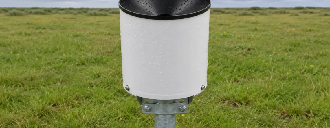
If a tipping bucket rain gauge reads low, check three points in order. First, make sure rain can reach the collector and drain into the buckets. Then verify that a measured flow produces the expected number of physical tips. Finally, confirm that the logger records each tip and applies the right depth per tip. A gauge can pass a slow water check and still miss rain in gusty weather or understate the peak of a downpour.
Start with the symptom. A low daily total, a short burst missing from the intensity chart, and a pulse recorded after the rain stopped call for different checks. Keep the raw counts or timestamps and define the time period you are comparing before changing the gauge. That gives you a record against which to judge each change.
What a tipping bucket rain gauge measures
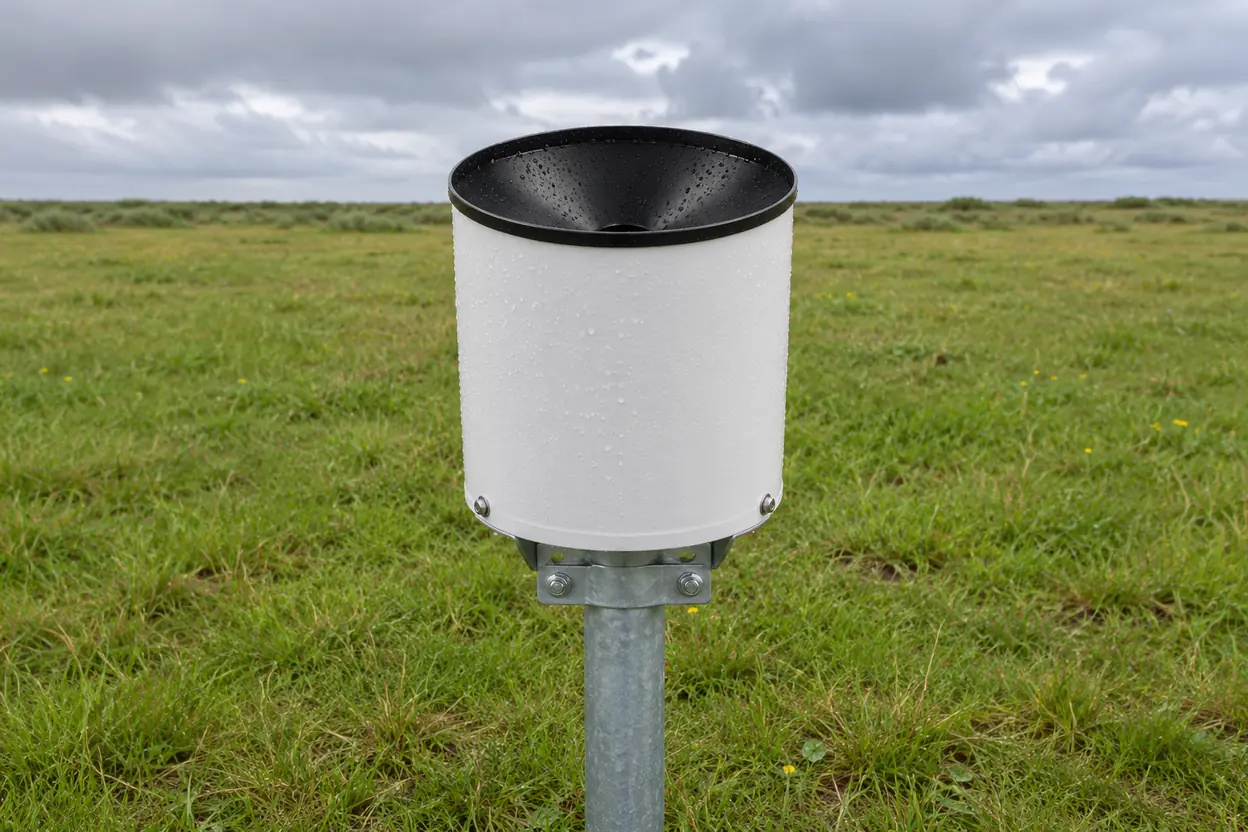
Rain enters a collector with a known opening area and drains through a funnel into one half of a two-compartment rocker. When enough water fills the raised compartment, the rocker pivots. The filled side empties and the other side moves under the funnel. A common design passes a magnet by a reed switch as the rocker tips, briefly closing the circuit. A compatible logger counts that closure or records its time. The gauge can operate repeatedly because the water exits through drains at the bottom. Onset's RG3 and RG3-M manual illustrates this arrangement.
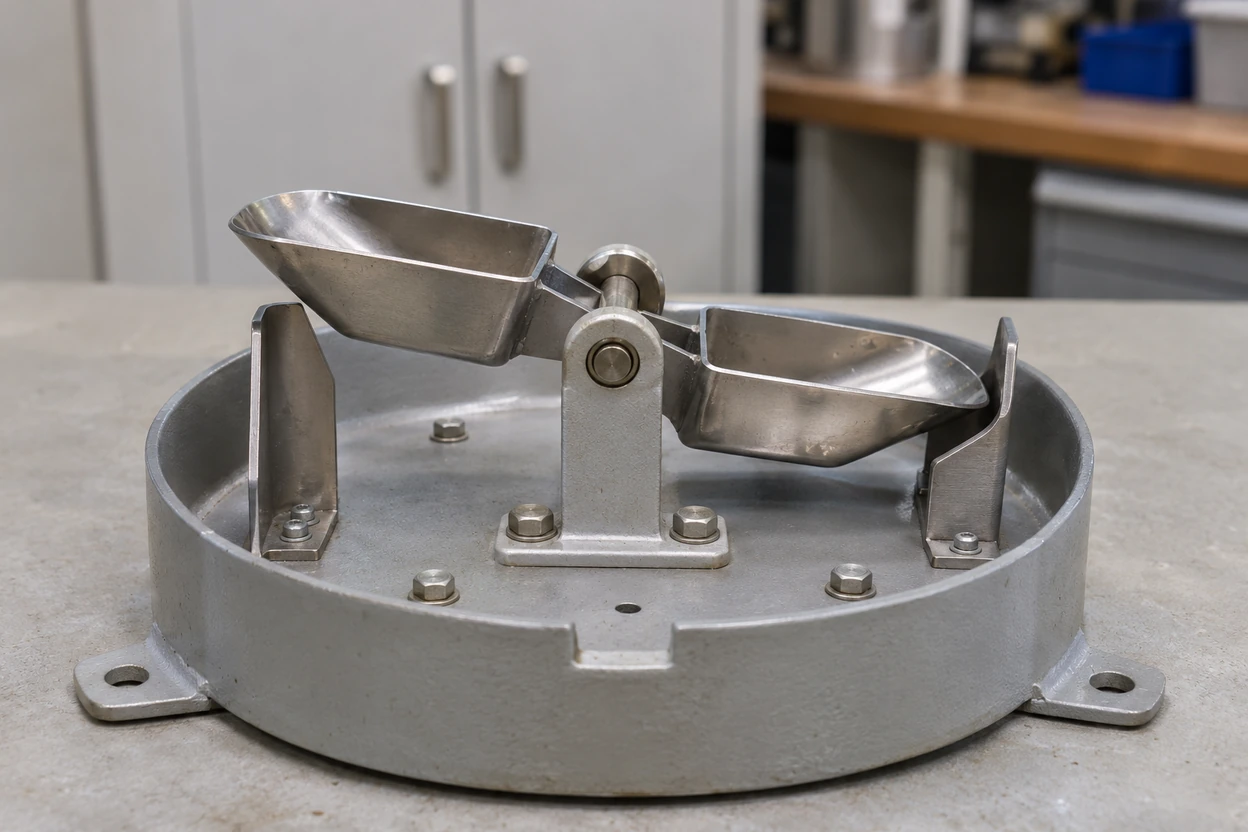
The two cups share a pivot and take turns receiving water. This illustration shows the exposed mechanism. The collector and funnel sit above it in operation.
The reported depth is the number of valid tips multiplied by the nominal depth per tip. For a gauge set to 0.20 mm per tip, 25 tips report 5.0 mm. The nominal increment describes the size of the measurement step. Accuracy also depends on how much rain enters the opening, how the rocker responds to flow and whether the logger counts correctly.
For a circular opening, calculate the area from its effective receiving diameter, which can differ from the body diameter. Divide captured volume in cubic millimeters by this area in square millimeters to obtain equivalent depth in millimeters. One milliliter equals 1,000 cubic millimeters. A hypothetical 200 mm receiving diameter gives an area of about 31,416 mm². At 0.20 mm per tip, the geometric equivalent is about 6.28 mL per tip. Use the manufacturer's stated increment and test procedure when configuring or checking a real gauge.
A partial fill explains why the first recorded tip can come after the rain starts. At the end of the event, water can remain in one side without making a pulse. It may contribute to the first tip in the next shower, or evaporate in the meantime. Two intervals with the same amount of rain can therefore have different counts when the initial fill is different. An empty event record means no tip reached the logger during that period. It cannot tell you how much water remained below the tipping threshold.
Where and how to install the gauge
Look for a site that represents the area whose rainfall you need to measure. In an orchard, a collector under a canopy measures a mixture of throughfall and drips rather than open rainfall. A gauge by a wall can sit in a rain shadow in one wind direction and receive concentrated runoff in another. An exposed roof or ridge can be windier than the field you want to represent. Walk the site with likely storm directions in mind and account for full tree foliage, seasonal crop growth and new equipment that might obstruct the opening.
Give the opening clearance without putting the gauge high in the wind. Wind can accelerate and deflect around the collector, carrying some drops past the opening. The NOAA/NWS cooperative station manual gives an optimal separation of at least twice the height of nearby obstructions for its siting context and emphasizes the increase in undercatch at windier locations. Use your own monitoring program's siting requirements where specified. On a sloped site, assess the angle of nearby objects as seen from the collector as well as their distance on the map. Field comparisons have found that mounting height and collector shape can affect wind-induced losses, so a percentage measured on another gauge or site cannot reliably correct yours. Field study by Pollock and colleagues.
Choose a stable support and keep the intake and drains clear. A short, rigid support can limit exposure while keeping the opening above local splash, vegetation and plausible standing water. Follow the required installation height and the manufacturer's mounting detail. Avoid sprinkler spray, irrigation booms, roof runoff, pavement splash and the discharge of another gauge. Keep the outlet open so drained water can leave freely. A separate mount is often practical if the station's anemometer needs a higher, more exposed position. The automatic weather station overview shows how the rain channel fits with other sensors, power and data collection.
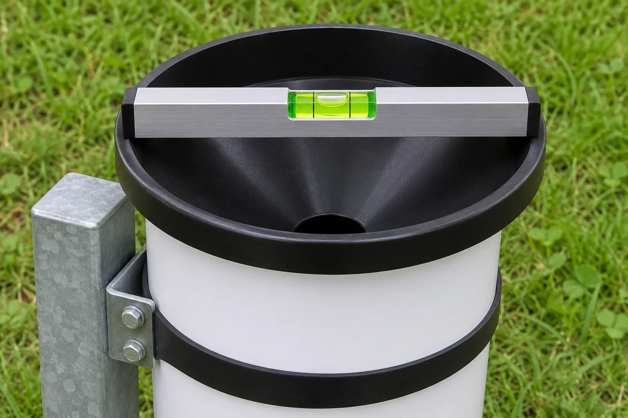
Use the leveling reference specified for your gauge. Some models provide an internal bubble level at the bucket assembly.
Level the gauge after tightening the mount. Use the specified bubble or machined reference, and verify both axes if the instructions call for it. A tilt can change the water needed to tip each side. Even if the total over many tips looks reasonable, unequal cups can distort short-interval intensity. Recheck level after the first service visit or after work on the mast. Remove any transport restraint according to the installation manual and check that the rocker moves freely through its full travel. Leave clearance to take the cover off, inspect the funnel and service the logger without bending the bracket.
Record the receiving height, nearby obstacles, gauge and logger serial numbers, multiplier and units, as well as the date and a few site photographs. This matters when comparing data before and after a crop grows, a pole shifts or a gauge moves. The USGS precipitation data policy provides an example of how a monitoring program documents siting and maintenance for a representative time series.
Commission the pulse input and rainfall intensity
Work from the raw acquisition channel out to the dashboard. For a passive reed-switch gauge, verify that the logger input supports switch closures and wire it according to the drawings for that specific gauge and logger combination. Other designs can have a powered output, an internal logger or an interface that reports a digital total. Verify the electrical interface before choosing an input mode. The Campbell Scientific TB4 and TB4MM manual shows how wiring and pulse settings depend on the logger and how the conversion differs between the two gauge models.
If the instrument instructions allow it, produce several deliberate tips and compare the physical count with the raw logger count. For example, ten clear tips should give ten new records or a ten-count increase. Look for missed or doubled counts as well as a complete absence of data. If the counts differ, check terminals, the active input channel, the input mode and the manufacturer's recommendations for switch bounce and pulse duration. A test at widely spaced intervals proves the basic connection. Confirm the input's pulse-width and rate limits for the shortest intervals the installation is expected to encounter.
Once the counts match, check the conversion. A model marked 0.01 inch per tip delivers 0.254 mm per tip. A model marked 0.20 mm per tip has a different increment. If a 0.01-inch gauge is accidentally programmed as 0.20 mm per tip, 100 correct pulses report 20.0 mm instead of 25.4 mm. The resulting shortfall is about 21%, independent of the true rainfall intensity as long as the physical tips are correct. Check that conversion is applied only once. Some instruments or gateways already provide depth in engineering units.
Choosing a reporting interval
For a fixed interval, divide the interval depth by the interval duration in hours. A 0.20 mm gauge that logs 15 tips in five minutes reports 3.0 mm for that period, equivalent to a mean intensity of 36 mm/h. A chart that shows 36 mm/h is describing the five-minute average expressed on an hourly scale. The measured depth remains 3.0 mm.
| Available record | Calculation | How to interpret it |
|---|---|---|
| Event count | Tips × depth per tip | Accumulation over the selected period |
| Fixed time bin | Bin depth ÷ bin duration | Average rate over a known time window |
| Event timestamps | One tip increment ÷ inter-tip duration | Estimate across the elapsed time between two tips |
A short bin preserves more timing detail but shows larger jumps from one tip. With 0.20 mm per tip, a one-minute bin advances in 12 mm/h steps. A bin can show zero followed by 12 mm/h during steady light rain simply because the bucket finished filling in the second minute. A longer interval smooths this behavior, while also reducing the apparent height of short peaks. Publish the interval with the rate so users can compare like with like.
With event timestamps, check clock resolution and sync. If adjacent tips appear six seconds apart, 0.20 mm divided by that duration is 120 mm/h. With timestamps reported in whole seconds, displayed gaps of five or seven seconds give 144 or about 103 mm/h. That sensitivity can dominate an isolated peak. The time between tips can also span a pause between showers, making the estimate an average over both the rain and the pause. Treat a first tip with no relevant preceding tip and duplicate timestamps explicitly instead of interpreting them as ordinary rate estimates.
Make sure the published series matches the logger
Check the first and last interval, time zone, and whether interval labels identify the start or end of the window. Decide where to put a pulse exactly at a boundary so it appears once. If data come from a cumulative counter, account for restarts and documented rollovers before taking differences. Preserve raw counts and identify missing time separately from valid zero-count periods. A dead logger can look like several dry hours if a reporting system fills blank records with zero.
Check that service tips do not enter the weather record. Log their timestamps and mark the affected data as maintenance. Retain the original acquisition so you can distinguish a maintenance correction, a missed upload and a true change in rainfall. When the gateway and logger disagree, compare raw records before replacing the gauge.
Check calibration at slow flow and across rain rates
A water check is useful only when you know what it measures. A known slow dose checks nominal depth response with limited high-rate effects. A dynamic calibration compares the gauge against a measured reference at several steady flow rates. The WMO guide to precipitation measurement, chapter 6 and annex 6.C, treats steady reference flow as the basis of dynamic calibration.
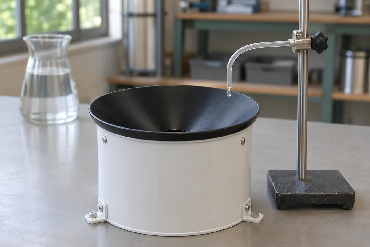
Apply water at the location and rate prescribed by the method. This illustration shows water entering the collector. Reference volume and time must be measured separately.
Start with the manufacturer's slow check
With the gauge level, inspect the collector, screen, outlet and rocker. Clean only as instructed and note whether the test starts dry, pre-wetted or from a defined point in the tip cycle. Follow the manufacturer's conditions for water dose, application time and expected count. Where accessible, compare physical tips and logged tips during the same check. A hand-poured cup can reveal that water reaches the buckets, but a brief surge cannot reproduce a specified flow test.
As a model-specific example, the Onset RG3-M manual specifies 373 mL through a slow field-check container, with at least an hour for the dose to run out and a target of 100 tips within two tips. Its RG3 sibling uses 473 mL and reports 0.01 inch per tip. The Campbell TB4 family manual describes a different volume and application period and recommends returning a failing instrument for recalibration. Before changing adjustment screws, identify the model and determine whether its instructions permit field adjustment. Re-run the prescribed check after an authorized adjustment and preserve both results.
With a short dose, one uncounted end fraction can be a large share of the test. The starting condition, repeatability and manufacturer tolerance matter more than whether one short run happened to yield an exact integer count. When comparing successive runs, use the same setup and verify that water is not lingering in a blocked screen or delivery tube. A repeat at the same setting can reveal inconsistent tip thresholds or a delivery problem that a single count conceals.
Use measured flow to investigate a heavy-rain shortfall
During a tip, the mechanism takes time to empty and move the other side into position. Some incoming water can join the bucket already discharging, so the same count can represent more water entering the collector at high flow. The shape and magnitude of this error depend on the mechanism and flow path. A siphon can regulate water delivery to the bucket but can also smooth very brief peaks. Other designs use mechanical compensation or a model-specific software correction. Very low flow and transitions between drops and a stream can also behave differently. The WMO guide describes intensity-dependent errors, including possible overestimation at low rates for uncorrected gauges. A bias measured at one flow rate cannot characterize the entire range.
For a multi-rate check, deliver a stable flow with suitable calibrated equipment and verify the actual delivery independently, for example by collecting and weighing the water over a timed interval. Select reference rates that span the conditions relevant to the station and that stay within the instrument and test equipment's rated range. Let delivery settle, use a consistent timing or tip-count protocol for each point, and collect enough tips to limit the influence of a single interval boundary. Record repeats, measured volume and duration, physical and logged counts, level, serial number and any compensation already applied.
A proper comparison uses the same period or the same defined span of tips for the reference and gauge. For example, a steady-flow method can measure elapsed time from one tip to a later tip, so the reference depth applies over a known number of complete inter-tip intervals. A fixed-time test must account for initial and final fill states and any water still moving through the collector at the cutoff. Treat a discrepancy near the size of a tip in light of those boundaries and the uncertainty of the reference flow.
Worked example with a 200 mm receiving diameter
Consider an illustrative gauge with a 0.20 mm nominal increment and a 31,416 mm² opening. A steady reference intensity of 60 mm/h corresponds to 1.00 mm/min. Through this opening, that is 31.42 mL/min. Over 12 minutes the reference water volume is about 377 mL, equivalent to 12.00 mm. Suppose the test yields 56 tips after accounting for timing and fill conditions, and the logger captures all 56.
| Quantity | Reference | Gauge record |
|---|---|---|
| Duration | 12 min | 12 min |
| Equivalent depth | 12.00 mm | 56 × 0.20 = 11.20 mm |
| Average intensity | 60.0 mm/h | 56.0 mm/h |
| Error relative to reference depth | — | (11.20 − 12.00) ÷ 12.00 = −6.67% |
The matched physical and logged counts would locate this run's shortfall upstream of the logger. The next question is whether the result repeats and changes with flow. If it does, compare with the gauge's specified performance or arrange a documented calibration. Keep any fitted relationship with the tested instrument and range. Preserve the uncorrected series alongside derived values and avoid applying a second correction to data the instrument has already compensated.
Where a validated model supplies a corrected intensity, store it as a separate quantity with its averaging window, calibration revision and applicable rate range. If the method also supplies corrected depth, aggregate that output according to the documented algorithm. Retain the nominal count-based depth, since it is directly reproducible from the pulses and shows how much the processing changed the result. A software adjustment for bucket motion only addresses the measured response to water delivered through the collector. Field catch requires separate evidence.
Why a tipping bucket gauge reads low in the field
When the bench response looks sound, compare the field conditions with the test conditions. A controlled water supply begins with water already entering the collector. Outdoor measurements first depend on the catch. Gusts can reduce catch, while trees or nearby walls can alter what reaches the rim. Funnel residue, a partly blocked screen or insects can hold water upstream of the buckets. Some water can drain later and produce tips after the storm, while some can be lost through evaporation or overflow.
Field and bench checks complement one another. For example, if counts agree in a controlled test and rain totals agree with a co-located manual gauge during calm storms, a discrepancy during windy storms makes exposure worth investigating. If physical and logged counts diverge at the same reference flow that gives the apparent shortfall, resolve the count mismatch and repeat the test before evaluating the mechanical response. With only a dashboard total, these two patterns can look identical.
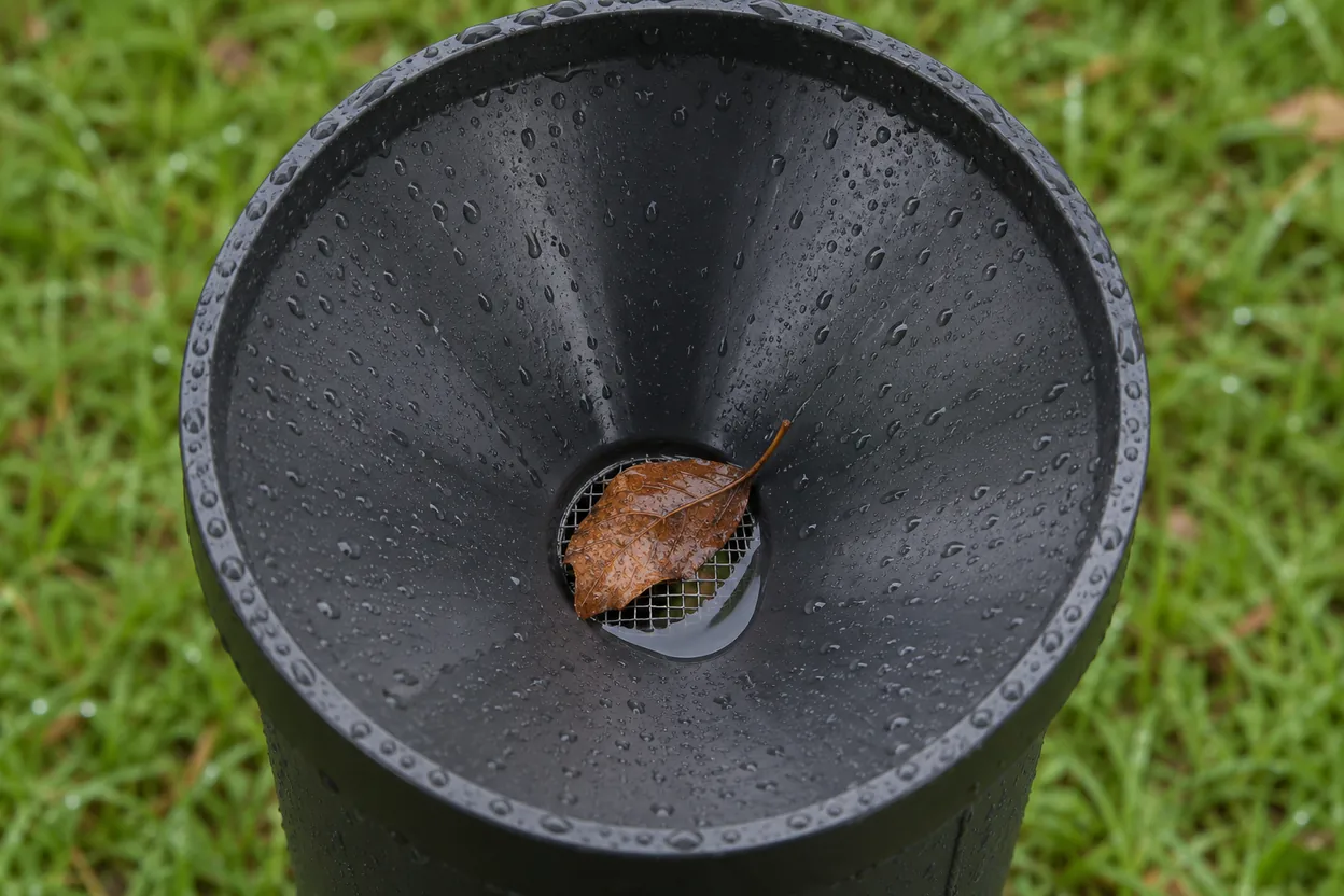
Partial blockage can shift the timing of the record even when water eventually reaches the buckets.
| Observed pattern | Start with this check | What the result can separate |
|---|---|---|
| Nearly constant proportional shortfall across events | Compare physical tips, logger counts, model increment and output units | Incorrect scaling versus a physical response issue |
| Bench check passes, but windy events read low | Review exposure and compare with a nearby, similarly exposed reference over the same interval | Field catch effects versus a bench-measurable fault |
| Heavy rain reads low even under controlled flow | Repeat at several measured flow rates and count tips both ways | Rate-dependent mechanics versus missed input events |
| Total is close, but the displayed peak is lower | Align bin widths, clocks and averaging methods | Reporting differences versus an instrument response difference |
| Drizzle shows no tips, or a few tips arrive late | Inspect the screen and flow path, then consider the depth increment and residual fill | Delayed or blocked flow versus normal discrete response |
| Rain appears on a dry day | Inspect mount vibration, irrigation, switch bounce and service history | False mechanical tips, electrical doubles or real water from a local source |
A nearby standard manual gauge is helpful for checking event totals. Its event total alone cannot establish the height or timing of a short rain-rate peak. That comparison requires a reference with suitable time response and a comparable averaging window. It still has its own exposure and measurement uncertainty. Place the instruments close enough to experience comparable weather while avoiding mutual obstruction and splash, and match the comparison interval. In particular, align the manual gauge's reading time with the logger total. An airport report, radar estimate or station across town gives context, but local showers can differ over short distances. Use a close reference and repeated events before attributing the difference to instrument bias.
When servicing the station, inspect the catch rim, drain screen, any siphon, the bucket pivot and drainage fittings as the manufacturer directs. Confirm level, gently verify motion if permitted, and record what changed. Compare the next scheduled check with the previous result. If leaf fall, insects or site work repeatedly affects the gauge, adapt the visit schedule to the pattern. Keep a record of relocations, replaced collectors, changes in depth per tip and logger settings so the historical rainfall series can be interpreted.
Frequently asked questions
Why does my gauge register less rain than a nearby weather station?
First compare the same period, time zone and units. Then consider distance and exposure. A shower can vary across a site, and the other gauge might have a different height, shelter or collector shape. If several paired events at the same site show the same shortfall, use a physical-tip and logger-count comparison followed by a measured water check to locate the discrepancy.
How often should I check calibration?
Use the interval and procedure for the model and monitoring program. The Onset RG3 and RG3-M manual calls for annual field calibration. Also check after work that could affect performance, such as a moved mount, a replaced collector or damage to the rocker. Periodic checks are easier to interpret when the test setup, conditions and previous results are documented.
Can I use a bottle with a small hole to calibrate the gauge?
A slow bottle can be appropriate when the manufacturer specifies that approach and you can measure the dose and verify the delivery time. It is usually a one-condition field check. For a rate-dependent characterization, use measured steady flows and document each reference point. Gravity flow from an ordinary container can vary as its water level falls.
Is 0.20 mm per tip the same as 0.01 inch per tip?
No. One hundred tips at 0.20 mm represent 20.0 mm. One hundred tips at 0.01 inch represent 1 inch, or 25.4 mm. Use the increment on the instrument documentation or calibration record. The display units can be changed independently of the gauge's physical tipping threshold.
Will a heated tipping bucket measure snowfall?
A model designed for winter use can melt captured snow and report its liquid equivalent when the meltwater reaches the buckets. Gauge catch, wind and melt timing affect that result. An unheated liquid-rain gauge can retain snow or ice and later register melt as tips, which shifts the apparent timing. For mixed or frozen precipitation, select the instrument and exposure required for the observing program. USGS precipitation data policy.
How can I tell whether a low peak comes from the gauge or from averaging?
Recalculate both data sets over identical windows with synchronized clocks. If the gap shrinks when the windows match, the original comparison was sensitive to reporting interval. If the gap persists at high intensity, use a controlled flow check and compare physical tips with raw logger pulses. That separates a rate-dependent mechanical response from missed counts before either is mixed with the effects of field exposure.







Leave a Reply